Ich bin KI-Forscher, also beschäftige ich mich hauptsächlich mit Daten. viel davon.
Mit mehr als 2,5 Exabyte an Daten, die jeden Tag generiert werden , ist es nicht verwunderlich, dass diese Daten irgendwo gespeichert werden müssen, wo wir bei Bedarf darauf zugreifen können.
Dieser Artikel führt Sie durch ein hackbares Cheatsheet, um Sie schnell mit SQL zum Laufen zu bringen.
Was ist SQL?
SQL steht für Structured Query Language. Es ist eine Sprache für relationale Datenbankverwaltungssysteme. SQL wird heute zum Speichern, Abrufen und Bearbeiten von Daten in relationalen Datenbanken verwendet.
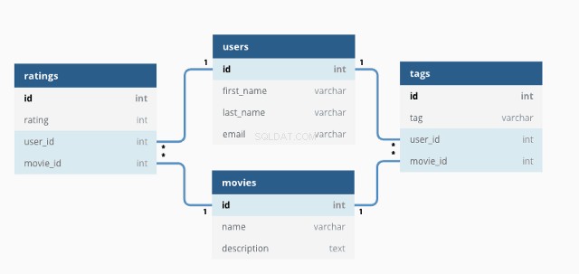
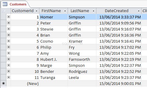
So sieht eine einfache relationale Datenbank aus:
Mithilfe von SQL können wir mit der Datenbank interagieren, indem wir Abfragen schreiben
So sieht eine Beispielabfrage aus:
SELECT * FROM customers;
Mit diesem SELECT -Anweisung wählt die Abfrage alle aus die Daten aus allen Spalten in der Kundentabelle und gibt Daten wie folgt zurück:
Das Sternchen-Platzhalterzeichen (*) bezieht sich auf „alle “ und wählt alle aus die Zeilen und Spalten. Wir können es stattdessen durch spezifische Spaltennamen ersetzen – hier werden nur diese Spalten von der Abfrage zurückgegeben
SELECT FirstName, LastName FROM customers;
Hinzufügen eines WHERE -Klausel können Sie filtern, was zurückgegeben wird:
SELECT * FROM customers WHERE age >= 30 ORDER BY age ASC;Diese Abfrage gibt alle Daten aus der Produkttabelle mit einem Alter zurück Wert größer als 30.
Die Verwendung von ORDER BY Schlüsselwort bedeutet lediglich, dass die Ergebnisse anhand der Altersspalte vom niedrigsten zum höchsten Wert geordnet werden
Mit INSERT INTO -Anweisung können wir neue Daten zu einer Tabelle hinzufügen. Hier ist ein einfaches Beispiel für das Hinzufügen eines neuen Benutzers zur Kundentabelle:
INSERT INTO customers(FirstName, LastName, address, email)
VALUES ('Jason', 'Dsouza', 'McLaren Vale, South Australia', 'test@fakeGmail.com');
Natürlich zeigen diese Beispiele nur eine sehr kleine Auswahl dessen, was die SQL-Sprache alles kann. Wir werden in diesem Leitfaden mehr darüber erfahren.
Warum SQL lernen?
Wir leben im Zeitalter von Big Data, in dem Daten ausgiebig genutzt werden, um Erkenntnisse zu gewinnen und Strategien, Marketing, Werbung und eine Vielzahl anderer Vorgänge zu informieren.
Große Unternehmen wie Google, Amazon und AirBnb nutzen große, relationale Datenbanken als Grundlage für die Verbesserung des Kundenerlebnisses. Das Verständnis von SQL ist nicht nur für Data Scientists und Analysten, sondern für alle eine großartige Fähigkeit.
Wie denkst du, dass du plötzlich eine YouTube-Werbung für Schuhe bekommen hast, als du noch vor ein paar Minuten deine Lieblingsschuhe gegoogelt hast? Das ist SQL (oder eine Form von SQL) bei der Arbeit!
SQL vs. MySQL
Bevor wir fortfahren, möchte ich nur ein oft verwirrtes Thema klären – den Unterschied zwischen SQL und MySQL. Wie sich herausstellt, sind sie es nicht dasselbe!
SQL ist eine Sprache, während MySQL ein System zur Implementierung von SQL ist.
SQL skizziert die Syntax, mit der Sie Abfragen schreiben können, die relationale Datenbanken verwalten.
MySQL ist ein Datenbanksystem die auf einem Server läuft. Es erlaubt Ihnen, Abfragen mit SQL-Syntax zu schreiben, um MySQL-Datenbanken zu verwalten.
Neben MySQL gibt es noch andere Systeme, die SQL implementieren. Einige der beliebtesten sind:
- SQLite
- Oracle-Datenbank
- PostgreSQL
- Microsoft SQL-Server
So installieren Sie MySQL
In den meisten Fällen ist MySQL die bevorzugte Wahl für ein Datenbankverwaltungssystem. Viele beliebte Content-Management-Systeme (wie Wordpress) verwenden standardmäßig MySQL, daher kann die Verwendung von MySQL zur Verwaltung dieser Anwendungen eine gute Idee sein.
Um MySQL verwenden zu können, müssen Sie es auf Ihrem System installieren:
Installieren Sie MySQL unter Windows
Die empfohlene Methode zur Installation von MySQL unter Windows ist die Verwendung des MSI-Installationsprogramms von der MySQL-Website.
Diese Ressource führt Sie durch den Installationsprozess.
Installieren Sie MySQL unter macOS
Unter macOS beinhaltet die Installation von MySQL auch das Herunterladen eines Installationsprogramms.
Diese Ressource führt Sie durch den Installationsprozess.
Wie man MySQL verwendet
Da MySQL jetzt auf Ihrem System installiert ist, empfehle ich Ihnen, eine Art SQL-Verwaltungsanwendung zu verwenden um die Verwaltung Ihrer Datenbanken zu vereinfachen.
Es stehen viele Apps zur Auswahl, die größtenteils die gleiche Aufgabe erfüllen, also liegt es an Ihren persönlichen Vorlieben, welche Sie verwenden möchten:
- MySQL Workbench entwickelt von Oracle
- phpMyAdmin (arbeitet im Webbrowser)
- HeidiSQL (Empfohlen für Windows)
- Sequel Pro (Empfohlen für macOS)
Wenn Sie bereit sind, Ihre eigenen SQL-Abfragen zu schreiben, sollten Sie erwägen, Dummy-Daten zu importieren, anstatt Ihre eigene Datenbank zu erstellen.
Hier sind einige Dummy-Datenbanken, die kostenlos heruntergeladen werden können.
SQL-Cheatsheet – das Sahnehäubchen
SQL-Schlüsselwörter
Hier finden Sie eine Sammlung von Schlüsselwörtern, die in SQL-Anweisungen verwendet werden, eine Beschreibung und gegebenenfalls ein Beispiel. Einige der fortgeschritteneren Keywords haben einen eigenen Abschnitt.
Wenn MySQL neben einem Beispiel erwähnt wird, bedeutet dies, dass dieses Beispiel nur auf MySQL-Datenbanken anwendbar ist (im Gegensatz zu anderen Datenbanksystemen).
ADD -- Adds a new column to an existing table

ADD CONSTRAINT -- Creates a new constraint on an existing table, which is used to specify rules for any data in the table.

ALTER TABLE -- Adds, deletes or edits columns in a table. It can also be used to add and delete constraints in a table, as per the above.

ALTER COLUMN -- Changes the data type of a table’s column.

ALL -- Returns true if all of the subquery values meet the passed condition.

AND -- Used to join separate conditions within a WHERE clause.

ANY -- Returns true if any of the subquery values meet the given condition.

AS -- Renames a table or column with an alias value which only exists for the duration of the query.

ASC -- Used with ORDER BY to return the data in ascending order.

BETWEEN -- Selects values within the given range.

CASE -- Changes query output depending on conditions.

CHECK -- Adds a constraint that limits the value which can be added to a column.

CREATE DATABASE -- Creates a new database.

CREATE TABLE -- Creates a new table.

DEFAULT -- Sets a default value for a column

DELETE -- Delete data from a table.

DESC -- Used with ORDER BY to return the data in descending order.

DROP COLUMN -- Deletes a column from a table.

DROP DATABASE -- Deletes the entire database.

DROP DEAFULT -- Removes a default value for a column.

DROP TABLE -- Deletes a table from a database.

EXISTS -- Checks for the existence of any record within the subquery, returning true if one or more records are returned.

FROM -- Specifies which table to select or delete data from.

IN --  Used alongside a WHERE clause as a shorthand for multiple OR conditions.

INSERT INTO -- Adds new rows to a table.

IS NULL -- Tests for empty (NULL) values.

IS NOT NULL -- The reverse of NULL. Tests for values that aren’t empty / NULL.

LIKE -- Returns true if the operand value matches a pattern.

NOT -- Returns true if a record DOESN’T meet the condition.

OR -- Used alongside WHERE to include data when either condition is true.

ORDER BY -- Used to sort the result data in ascending (default) or descending order through the use of ASC or DESC keywords.

ROWNUM -- Returns results where the row number meets the passed condition.

SELECT -- Used to select data from a database, which is then returned in a results set.

SELECT DISTINCT -- Sames as SELECT, except duplicate values are excluded.

SELECT INTO -- Copies data from one table and inserts it into another.

SELECT TOP -- Allows you to return a set number of records to return from a table.

SET -- Used alongside UPDATE to update existing data in a table.

SOME -- Identical to ANY.

TOP -- Used alongside SELECT to return a set number of records from a table.

TRUNCATE TABLE -- Similar to DROP, but instead of deleting the table and its data, this deletes only the data.

UNION -- Combines the results from 2 or more SELECT statements and returns only distinct values.

UNION ALL -- The same as UNION, but includes duplicate values.

UNIQUE -- This constraint ensures all values in a column are unique.

UPDATE -- Updates existing data in a table.

VALUES -- Used alongside the INSERT INTO keyword to add new values to a table.

WHERE -- Filters results to only include data which meets the given condition.
Kommentare in SQL
Kommentare ermöglichen es Ihnen, Abschnitte Ihrer SQL-Anweisungen zu erklären, ohne direkt ausgeführt zu werden.
In SQL gibt es zwei Arten von Kommentaren, einzeilig und mehrzeilig.
Einzeilige Kommentare in SQL
Einzeilige Kommentare beginnen mit „- -“. Jeglicher Text nach diesen 2 Zeichen bis zum Ende der Zeile wird ignoriert.
-- This part is ignored

SELECT * FROM customers;
Mehrzeilige Kommentare in SQL
Mehrzeilige Kommentare beginnen mit /* und enden mit */. Sie erstrecken sich über mehrere Zeilen, bis die Schlusszeichen gefunden sind.
/*

This is a multiline comment.
It can span across multiple lines.

*/

SELECT * FROM customers;

/*

This is another comment.
You can even put code within a comment to prevent its execution

SELECT * FROM icecreams;

*/
Datentypen in MySQL
Wenn Sie eine neue Tabelle erstellen oder eine vorhandene bearbeiten, müssen Sie den Datentyp angeben, den jede Spalte akzeptiert.
In diesem Beispiel werden Daten an id übergeben Spalte muss ein Int (Ganzzahl) sein, während FirstName Spalte hat einen VARCHAR Datentyp mit maximal 255 Zeichen.
CREATE TABLE customers(
id int,
FirstName varchar(255)
);
1. String-Datentypen
CHAR(size) -- Fixed length string which can contain letters, numbers and special characters. The size parameter sets the maximum string length, from 0 – 255 with a default of 1.

VARCHAR(size) -- Variable length string similar to CHAR(), but with a maximum string length range from 0 to 65535.

BINARY(size) -- Similar to CHAR() but stores binary byte strings.

VARBINARY(size) -- Similar to VARCHAR() but for binary byte strings.

TINYBLOB -- Holds Binary Large Objects (BLOBs) with a max length of 255 bytes.

TINYTEXT -- Holds a string with a maximum length of 255 characters. Use VARCHAR() instead, as it’s fetched much faster.

TEXT(size) -- Holds a string with a maximum length of 65535 bytes. Again, better to use VARCHAR().

BLOB(size) -- Holds Binary Large Objects (BLOBs) with a max length of 65535 bytes.

MEDIUMTEXT -- Holds a string with a maximum length of 16,777,215 characters.

MEDIUMBLOB -- Holds Binary Large Objects (BLOBs) with a max length of 16,777,215 bytes.

LONGTEXT -- Holds a string with a maximum length of 4,294,967,295 characters.

LONGBLOB -- Holds Binary Large Objects (BLOBs) with a max length of 4,294,967,295 bytes.

ENUM(a, b, c, etc…) -- A string object that only has one value, which is chosen from a list of values which you define, up to a maximum of 65535 values. If a value is added which isn’t on this list, it’s replaced with a blank value instead.

SET(a, b, c, etc…) -- A string object that can have 0 or more values, which is chosen from a list of values which you define, up to a maximum of 64 values.
2. Numerische Datentypen
BIT(size) -- A bit-value type with a default of 1. The allowed number of bits in a value is set via the size parameter, which can hold values from 1 to 64.

TINYINT(size) -- A very small integer with a signed range of -128 to 127, and an unsigned range of 0 to 255. Here, the size parameter specifies the maximum allowed display width, which is 255.

BOOL -- Essentially a quick way of setting the column to TINYINT with a size of 1. 0 is considered false, whilst 1 is considered true.

BOOLEAN	-- Same as BOOL.

SMALLINT(size) -- A small integer with a signed range of -32768 to 32767, and an unsigned range from 0 to 65535. Here, the size parameter specifies the maximum allowed display width, which is 255.

MEDIUMINT(size) -- A medium integer with a signed range of -8388608 to 8388607, and an unsigned range from 0 to 16777215. Here, the size parameter specifies the maximum allowed display width, which is 255.

INT(size) -- A medium integer with a signed range of -2147483648 to 2147483647, and an unsigned range from 0 to 4294967295. Here, the size parameter specifies the maximum allowed display width, which is 255.

INTEGER(size) -- Same as INT.

BIGINT(size) -- A medium integer with a signed range of -9223372036854775808 to 9223372036854775807, and an unsigned range from 0 to 18446744073709551615. Here, the size parameter specifies the maximum allowed display width, which is 255.

FLOAT(p) -- A floating point number value. If the precision (p) parameter is between 0 to 24, then the data type is set to FLOAT(), whilst if it's from 25 to 53, the data type is set to DOUBLE(). This behaviour is to make the storage of values more efficient.

DOUBLE(size, d) -- A floating point number value where the total digits are set by the size parameter, and the number of digits after the decimal point is set by the d parameter.

DECIMAL(size, d) -- An exact fixed point number where the total number of digits is set by the size parameters, and the total number of digits after the decimal point is set by the d parameter.

DEC(size, d) -- Same as DECIMAL.
3. Datentypen für Datum/Uhrzeit
DATE -- A simple date in YYYY-MM–DD format, with a supported range from ‘1000-01-01’ to ‘9999-12-31’.

DATETIME(fsp) -- A date time in YYYY-MM-DD hh:mm:ss format, with a supported range from ‘1000-01-01 00:00:00’ to ‘9999-12-31 23:59:59’. By adding DEFAULT and ON UPDATE to the column definition, it automatically sets to the current date/time.

TIMESTAMP(fsp) -- A Unix Timestamp, which is a value relative to the number of seconds since the Unix epoch (‘1970-01-01 00:00:00’ UTC). This has a supported range from ‘1970-01-01 00:00:01’ UTC to ‘2038-01-09 03:14:07’ UTC.
By adding DEFAULT CURRENT_TIMESTAMP and ON UPDATE CURRENT TIMESTAMP to the column definition, it automatically sets to current date/time.

TIME(fsp) -- A time in hh:mm:ss format, with a supported range from ‘-838:59:59’ to ‘838:59:59’.

YEAR -- A year, with a supported range of ‘1901’ to ‘2155’.
SQL-Operatoren
1. Arithmetische Operatoren in SQL
+ -- Add
– -- Subtract
* -- Multiply
/ -- Divide
% -- Modulus
2. Bitweise Operatoren in SQL
& -- Bitwise AND
| -- Bitwise OR
^-- Bitwise XOR
3. Vergleichsoperatoren in SQL
= -- Equal to
> -- Greater than
< -- Less than
>= -- Greater than or equal to
<= -- Less than or equal to
<> -- Not equal to
4. Zusammengesetzte Operatoren in SQL
+= -- Add equals
-= -- Subtract equals
*= -- Multiply equals
/= -- Divide equals
%= -- Modulo equals
&= -- Bitwise AND equals
^-= -- Bitwise exclusive equals
|*= -- Bitwise OR equals
SQL-Funktionen
1. Zeichenfolgenfunktionen in SQL
ASCII -- Returns the equivalent ASCII value for a specific character.

CHAR_LENGTH -- Returns the character length of a string.

CHARACTER_LENGTH -- Same as CHAR_LENGTH.

CONCAT -- Adds expressions together, with a minimum of 2.

CONCAT_WS -- Adds expressions together, but with a separator between each value.

FIELD -- Returns an index value relative to the position of a value within a list of values.

FIND IN SET -- Returns the position of a string in a list of strings.

FORMAT -- When passed a number, returns that number formatted to include commas (eg 3,400,000).

INSERT -- Allows you to insert one string into another at a certain point, for a certain number of characters.

INSTR -- Returns the position of the first time one string appears within another.

LCASE -- Converts a string to lowercase.

LEFT -- Starting from the left, extracts the given number of characters from a string and returns them as another.

LENGTH -- Returns the length of a string, but in bytes.

LOCATE -- Returns the first occurrence of one string within another,

LOWER -- Same as LCASE.

LPAD -- Left pads one string with another, to a specific length.

LTRIM -- Removes any leading spaces from the given string.

MID -- Extracts one string from another, starting from any position.

POSITION -- Returns the position of the first time one substring appears within another.

REPEAT -- Allows you to repeat a string

REPLACE -- Allows you to replace any instances of a substring within a string, with a new substring.

REVERSE	-- Reverses the string.

RIGHT -- Starting from the right, extracts the given number of characters from a string and returns them as another.

RPAD -- Right pads one string with another, to a specific length.

RTRIM -- Removes any trailing spaces from the given string.

SPACE -- Returns a string full of spaces equal to the amount you pass it.

STRCMP -- Compares 2 strings for differences

SUBSTR -- Extracts one substring from another, starting from any position.

SUBSTRING -- Same as SUBSTR

SUBSTRING_INDEX	-- Returns a substring from a string before the passed substring is found the number of times equals to the passed number.

TRIM --	Removes trailing and leading spaces from the given string. Same as if you were to run LTRIM and RTRIM together.

UCASE -- Converts a string to uppercase.

UPPER -- Same as UCASE.
2. Numerische Funktionen in SQL
ABS -- Returns the absolute value of the given number.

ACOS -- Returns the arc cosine of the given number.

ASIN -- Returns the arc sine of the given number.

ATAN -- Returns the arc tangent of one or 2 given numbers.

ATAN2 -- Returns the arc tangent of 2 given numbers.

AVG -- Returns the average value of the given expression.

CEIL -- Returns the closest whole number (integer) upwards from a given decimal point number.

CEILING -- Same as CEIL.

COS -- Returns the cosine of a given number.

COT -- Returns the cotangent of a given number.

COUNT -- Returns the amount of records that are returned by a SELECT query.

DEGREES -- Converts a radians value to degrees.

DIV -- Allows you to divide integers.

EXP -- Returns e to the power of the given number.

FLOOR -- Returns the closest whole number (integer) downwards from a given decimal point number.

GREATEST -- Returns the highest value in a list of arguments.

LEAST -- Returns the smallest value in a list of arguments.

LN -- Returns the natural logarithm of the given number.

LOG -- Returns the natural logarithm of the given number, or the logarithm of the given number to the given base.

LOG10 -- Does the same as LOG, but to base 10.

LOG2 -- Does the same as LOG, but to base 2.

MAX -- Returns the highest value from a set of values.

MIN -- Returns the lowest value from a set of values.

MOD -- Returns the remainder of the given number divided by the other given number.

PI -- Returns PI.

POW -- Returns the value of the given number raised to the power of the other given number.

POWER -- Same as POW.

RADIANS -- Converts a degrees value to radians.

RAND -- Returns a random number.

ROUND -- Rounds the given number to the given amount of decimal places.

SIGN -- Returns the sign of the given number.

SIN -- Returns the sine of the given number.

SQRT -- Returns the square root of the given number.

SUM -- Returns the value of the given set of values combined.

TAN -- Returns the tangent of the given number.

TRUNCATE -- Returns a number truncated to the given number of decimal places.
3. Datumsfunktionen in SQL
ADDDATE -- Adds a date interval (eg: 10 DAY) to a date (eg: 20/01/20) and returns the result (eg: 20/01/30).

ADDTIME -- Adds a time interval (eg: 02:00) to a time or datetime (05:00) and returns the result (07:00).

CURDATE -- Gets the current date.

CURRENT_DATE -- Same as CURDATE.

CURRENT_TIME -- Gest the current time.

CURRENT_TIMESTAMP -- Gets the current date and time.

CURTIME -- Same as CURRENT_TIME.

DATE -- Extracts the date from a datetime expression.

DATEDIFF -- Returns the number of days between the 2 given dates.

DATE_ADD -- Same as ADDDATE.

DATE_FORMAT -- Formats the date to the given pattern.

DATE_SUB -- Subtracts a date interval (eg: 10 DAY) to a date (eg: 20/01/20) and returns the result (eg: 20/01/10).

DAY -- Returns the day for the given date.

DAYNAME -- Returns the weekday name for the given date.

DAYOFWEEK -- Returns the index for the weekday for the given date.

DAYOFYEAR -- Returns the day of the year for the given date.

EXTRACT -- Extracts from the date the given part (eg MONTH for 20/01/20 = 01).

FROM DAYS -- Returns the date from the given numeric date value.

HOUR -- Returns the hour from the given date.

LAST DAY -- Gets the last day of the month for the given date.

LOCALTIME -- Gets the current local date and time.

LOCALTIMESTAMP -- Same as LOCALTIME.

MAKEDATE -- Creates a date and returns it, based on the given year and number of days values.

MAKETIME -- Creates a time and returns it, based on the given hour, minute and second values.

MICROSECOND -- Returns the microsecond of a given time or datetime.

MINUTE -- Returns the minute of the given time or datetime.

MONTH -- Returns the month of the given date.

MONTHNAME -- Returns the name of the month of the given date.

NOW -- Same as LOCALTIME.

PERIOD_ADD -- Adds the given number of months to the given period.

PERIOD_DIFF -- Returns the difference between 2 given periods.

QUARTER -- Returns the year quarter for the given date.

SECOND -- Returns the second of a given time or datetime.

SEC_TO_TIME -- Returns a time based on the given seconds.

STR_TO_DATE -- Creates a date and returns it based on the given string and format.

SUBDATE -- Same as DATE_SUB.

SUBTIME -- Subtracts a time interval (eg: 02:00) to a time or datetime (05:00) and returns the result (03:00).

SYSDATE -- Same as LOCALTIME.

TIME -- Returns the time from a given time or datetime.

TIME_FORMAT -- Returns the given time in the given format.

TIME_TO_SEC -- Converts and returns a time into seconds.

TIMEDIFF -- Returns the difference between 2 given time/datetime expressions.

TIMESTAMP -- Returns the datetime value of the given date or datetime.

TO_DAYS -- Returns the total number of days that have passed from ‘00-00-0000’ to the given date.

WEEK -- Returns the week number for the given date.

WEEKDAY -- Returns the weekday number for the given date.

WEEKOFYEAR -- Returns the week number for the given date.

YEAR -- Returns the year from the given date.

YEARWEEK -- Returns the year and week number for the given date.
4. Verschiedene Funktionen in SQL
BIN -- Returns the given number in binary.

BINARY -- Returns the given value as a binary string.

CAST -- Converst one type into another.

COALESCE -- From a list of values, returns the first non-null value.

CONNECTION_ID -- For the current connection, returns the unique connection ID.

CONV -- Converts the given number from one numeric base system into another.

CONVERT -- Converts the given value into the given datatype or character set.

CURRENT_USER -- Returns the user and hostname which was used to authenticate with the server.

DATABASE -- Gets the name of the current database.

GROUP BY -- Used alongside aggregate functions (COUNT, MAX, MIN, SUM, AVG) to group the results.

HAVING -- Used in the place of WHERE with aggregate functions.

IF -- If the condition is true it returns a value, otherwise it returns another value.

IFNULL -- If the given expression equates to null, it returns the given value.

ISNULL -- If the expression is null, it returns 1, otherwise returns 0.

LAST_INSERT_ID -- For the last row which was added or updated in a table, returns the auto increment ID.

NULLIF -- Compares the 2 given expressions. If they are equal, NULL is returned, otherwise the first expression is returned.

SESSION_USER -- Returns the current user and hostnames.

SYSTEM_USER -- Same as SESSION_USER.

USER -- Same as SESSION_USER.

VERSION -- Returns the current version of the MySQL powering the database.
Platzhalterzeichen in SQL
In SQL sind Wildcards Sonderzeichen, die mit LIKE verwendet werden und NOT LIKE Schlüsselwörter. Dadurch können wir ziemlich effizient nach Daten mit ausgeklügelten Mustern suchen.
% -- Equates to zero or more characters.
-- Example: Find all customers with surnames ending in ‘ory’.
SELECT * FROM customers
WHERE surname LIKE '%ory';

_ -- Equates to any single character.
-- Example: Find all customers living in cities beginning with any 3 characters, followed by ‘vale’.
SELECT * FROM customers
WHERE city LIKE '_ _ _vale';

[charlist] -- Equates to any single character in the list.
-- Example: Find all customers with first names beginning with J, K or T.
SELECT * FROM customers
WHERE first_name LIKE '[jkt]%';
SQL-Schlüssel
In relationalen Datenbanken gibt es ein Konzept von primär und fremd Schlüssel. In SQL-Tabellen sind diese als Einschränkungen enthalten, wobei eine Tabelle einen Primärschlüssel, einen Fremdschlüssel oder beides haben kann.
1. Primärschlüssel in SQL
Mit einem Primärnamen kann jeder Datensatz in einer Tabelle eindeutig identifiziert werden. Sie können nur einen Primärschlüssel pro Tabelle haben, und Sie können diese Einschränkung jeder einzelnen oder Kombination von Spalten zuweisen. Das bedeutet jedoch, dass jeder Wert innerhalb dieser Spalte(n) eindeutig sein muss.
Typischerweise ist die ID-Spalte in einer Tabelle ein Primärschlüssel und wird normalerweise mit dem AUTO_INCREMENT gepaart Stichwort. Das heißt, der Wert erhöht sich automatisch, wenn neue Datensätze erstellt werden.
Beispiel (MySQL)
Erstellen Sie eine neue Tabelle und setzen Sie den Primärschlüssel auf die ID-Spalte.
CREATE TABLE customers (
id int NOT NULL AUTO_INCREMENT,
FirstName varchar(255),
Last Name varchar(255) NOT NULL,
address varchar(255),
email varchar(255),
PRIMARY KEY (id)
);
2. Fremdschlüssel in SQL
Sie können einen Fremdschlüssel auf eine oder mehrere Spalten anwenden. Sie verwenden es zum Verknüpfen 2 Tabellen zusammen in einer relationalen Datenbank.
Die Tabelle, die den Fremdschlüssel enthält, wird als Kind bezeichnet Schlüssel,
Die Tabelle, die den referenzierten (oder Kandidaten-) Schlüssel enthält, wird als Elternteil bezeichnet Tabelle.
Dies bedeutet im Wesentlichen, dass die Spaltendaten zwischen 2 Tabellen geteilt werden, da ein Fremdschlüssel auch verhindert, dass ungültige Daten eingefügt werden, die nicht auch in der übergeordneten Tabelle vorhanden sind.
Beispiel (MySQL)
Erstellen Sie eine neue Tabelle und wandeln Sie jede Spalte, die auf IDs in anderen Tabellen verweist, in Fremdschlüssel um.
CREATE TABLE orders (
id int NOT NULL,
user_id int,
product_id int,
PRIMARY KEY (id),
FOREIGN KEY (user_id) REFERENCES users(id),
FOREIGN KEY (product_id) REFERENCES products(id)
);
Indizes in SQL
Indizes sind Attribute, die Spalten zugewiesen werden können, nach denen häufig gesucht wird, um den Datenabruf zu einem schnelleren und effizienteren Prozess zu machen.
CREATE INDEX -- Creates an index named ‘idx_test’ on the first_name and surname columns of the users table. In this instance, duplicate values are allowed.
CREATE INDEX idx_test
ON users (first_name, surname);
CREATE UNIQUE INDEX -- The same as the above, but no duplicate values.
CREATE UNIQUE INDEX idx_test
ON users (first_name, surname);
DROP INDEX -- Removes an index.
ALTER TABLE users
DROP INDEX idx_test;
SQL-Joins
In SQL ein JOIN -Klausel wird verwendet, um ein Ergebnis zurückzugeben, das Daten aus mehreren Tabellen kombiniert, basierend auf einer gemeinsamen Spalte, die in beiden enthalten ist.
Es gibt eine Reihe verschiedener Joins, die Sie verwenden können:
- Innere Verknüpfung (Standard): Gibt alle Datensätze zurück, die übereinstimmende Werte in beiden Tabellen haben.
- Linker Beitritt: Gibt alle Datensätze aus der ersten Tabelle zusammen mit allen übereinstimmenden Datensätzen aus der zweiten Tabelle zurück.
- Right Join: Gibt alle Datensätze aus der zweiten Tabelle zusammen mit allen übereinstimmenden Datensätzen aus der ersten zurück.
- Vollständiger Beitritt: Gibt bei Übereinstimmung alle Datensätze aus beiden Tabellen zurück.
Eine gängige Methode zur Visualisierung der Funktionsweise von Joins sieht folgendermaßen aus:

SELECT orders.id, users.FirstName, users.Surname, products.name as ‘product name’
FROM orders
INNER JOIN users on orders.user_id = users.id
INNER JOIN products on orders.product_id = products.id;
Ansichten in SQL
Eine Ansicht ist im Wesentlichen eine SQL-Ergebnismenge, die in der Datenbank unter einem Label gespeichert wird, sodass Sie später darauf zurückgreifen können, ohne die Abfrage erneut ausführen zu müssen.
Diese sind besonders nützlich, wenn Sie eine kostspielige SQL-Abfrage haben, die Sie möglicherweise mehrmals benötigen. Anstatt es also immer wieder auszuführen, um denselben Ergebnissatz zu generieren, können Sie es einfach einmal tun und als Ansicht speichern.
So erstellen Sie Ansichten in SQL
So erstellen Sie eine Ansicht:
CREATE VIEW priority_users AS
SELECT * FROM users
WHERE country = ‘United Kingdom’;
Wenn Sie in Zukunft auf die gespeicherte Ergebnismenge zugreifen müssen, können Sie dies folgendermaßen tun:
SELECT * FROM [priority_users];Ersetzen von Ansichten in SQL
Mit dem CREATE OR REPLACE Befehl können Sie eine Ansicht wie folgt aktualisieren:
CREATE OR REPLACE VIEW [priority_users] AS
SELECT * FROM users
WHERE country = ‘United Kingdom’ OR country=’USA’;
So löschen Sie Ansichten in SQL
Um eine Ansicht zu löschen, verwenden Sie einfach DROP VIEW Befehl.
DROP VIEW priority_users;Schlussfolgerung
Die meisten Websites und Anwendungen verwenden auf die eine oder andere Weise relationale Datenbanken. Dies macht es äußerst wertvoll, SQL zu kennen, da Sie damit komplexere, funktionalere Systeme erstellen können.
Folgen Sie mir auf Twitter, um Updates zu zukünftigen Artikeln zu erhalten. Viel Spaß beim Lernen!